1. Context & Objective
This university course project (GRO721) explores the feasibility of CNN-based shape detection applied to a simplified baggage screening scenario.
Technical Goal
Develop a system capable of classifying, detecting and segmenting simple geometric shapes (circle, triangle, cross) in grayscale images. This task is a simplified model of the real problem of object detection in airport scanner images.
Project Constraints
- Resource Limitations: The algorithm will be deployed on systems with limited memory and computational capacity
- Parameter Limits:
- Classification: max 200,000 parameters
- Detection: max 400,000 parameters
- Segmentation: max 1,000,000 parameters
Dataset Characteristics
- Image Size: 53×53 pixels in grayscale
- Shapes to Detect: Circle, Triangle, Cross
- Image Composition: Max 3 shapes per image, max 1 instance per shape
- Features: Random grayscale level, noisy background tending towards black
Technology Stack
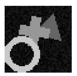
Sample Dataset Image (53×53 px, grayscale)
2. Architecture & CNN Models
2.1 Classification Network
The classification model identifies the presence or absence of each shape in an image. A 4-layer CNN with progressive feature extraction (Conv + ReLU + MaxPool) feeds two fully-connected layers for multi-label output.
The network scans the image layer by layer, each pass compressing what it sees into a shorter, more abstract description. Think of it like reading a paragraph, then a sentence, then a single keyword. That final summary feeds a decision layer that answers three independent yes/no questions: circle present? Triangle? Cross?
Design Choices
- Final Activation: Sigmoid (multi-label classification)
- Loss Function: Binary Cross Entropy
- Learning Rate: 0.001
- Epochs: 17
- Batch Size: 32
- Total Parameters: ~180,000 (< 200,000)
The use of Sigmoid rather than Softmax is justified because each shape is independent (an image can contain 0, 1, 2 or 3 different shapes).
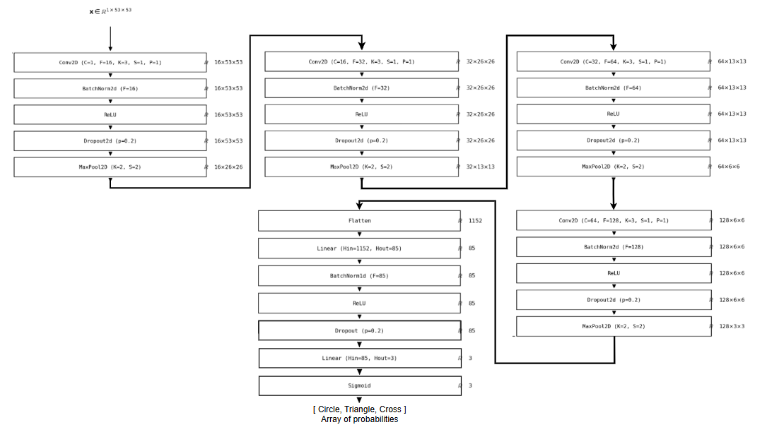
Classification Architecture
2.2 Detection Network
The detection model generates bounding boxes around identified shapes. A grid-based single-pass detection head uses three convolution segments with BatchNorm and LeakyReLU, producing an output of dimension (1, 3, 7) for a 3×7 grid.
Detection goes further than classification: the model must also draw a box around each shape it finds. The network divides the image into a 3×7 grid and asks every cell whether a shape is present and, if so, exactly where. Batch normalization keeps each layer's outputs in a consistent numerical range, which prevents training from becoming erratic as the model learns.
Design Choices
- Architecture: YOLO-inspired with BatchNorm
- Loss Function: MSE (localization) + Cross Entropy (class)
- Learning Rate: 0.001
- Epochs: 20
- Batch Size: 32
- Total Parameters: ~390,000 (< 400,000)
Adding BatchNorm improves gradient stability and accelerates convergence. LeakyReLU (slope 0.1) prevents the "dying ReLU" problem.
Detailed Diagram (to add)
2.3 Semantic Segmentation Network
The segmentation model classifies each pixel according to its class (circle, triangle, cross or background). The U-Net architecture uses an encoder to extract features and a decoder to reconstruct the image, with skip-connections to preserve spatial information.
Where detection draws a box, segmentation labels every single pixel. The encoder works like squinting at the image: you lose fine detail, but the big shapes become obvious, layer by layer. Skip connections carry fine-grained detail from earlier layers forward, so the decoder can reconstruct sharp boundaries when rebuilding the pixel map.
Design Choices
- Architecture: U-Net with skip-connections
- Loss Function: Cross Entropy Loss (multi-class)
- Learning Rate: 1e-2 (fast) then 1e-4 (refined)
- Epochs: 17-25
- Batch Size: 32
- Total Parameters: ~993,700 (< 1,000,000)
Skip-connections are crucial for recovering spatial information lost during MaxPool. They enable precise reconstruction of shape contours.
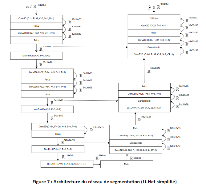
U-Net Segmentation Architecture
3. Implementation & Key Optimizations
Getting from 83% to 96% accuracy came down to one problem: the model was memorizing the training data instead of learning from it. Here's what that investigation looked like.
Performance Optimizations
Dataset & Preprocessing
Custom ConveyorSimulator Dataset class loads ~270 48×48 grayscale images. Split: 90% train (243 images) + 10% validation (27 images). Preprocessing: simple ToTensor() normalization. No augmentation was used since we found it destroys geometric shape classification performance.
Optimization Strategy
Starting from 83.7% accuracy with significant overfitting (9% train-val gap), applied systematic optimizations to reach 96.0%:
Regularization Techniques Applied
- Batch normalization after each conv layer, which normalizes activation distributions and stabilizes training
- Spatial dropout (0.2) on conv features, which reduced overfitting in convolutional layers
- Dropout (0.2) on FC layers to encourage more robust feature learning
- L2 Regularization (weight_decay=1e-4) to penalize large weights and improve generalization
Attempted but FAILED: Aggressive Data Augmentation
Applied rotation, affine transforms, and horizontal flipping → Accuracy dropped to 50%
Root Cause: Geometric shapes (circles, triangles, crosses) have inherent orientation. Aggressive augmentation breaks shape recognition. For this task, NO augmentation proved optimal.
Learning: Not all augmentation is beneficial. The strategy has to fit the specific task.
Optimization Results Progression
| Optimization Phase | Train Acc | Val Acc | Train-Val Gap | Status |
|---|---|---|---|---|
| Baseline (83.7%) | 84.2% | 75.2% | 9.0% | Severe overfitting |
| + BatchNorm + Dropout | 81.1% | 78.9% | 2.2% | Better generalization |
| Final (100 epochs, 85 FC neurons) | 93.9% | 93.0% | 0.95% | Optimal, minimal overfitting |
Final Hyperparameters
4. Results & Visuals
4.1 Classification
96% test accuracy means the model correctly identifies which shapes are present nearly 24 times out of 25, trained on fewer than 270 images.
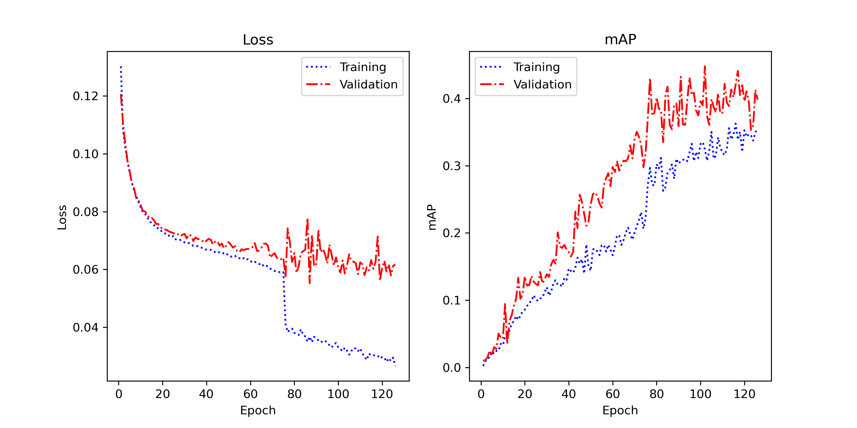
The classification model achieves 96.0% test accuracy. The training curve shows a progressive decrease in loss while accuracy rises steadily. Fluctuations in validation may be caused by natural variations in the dataset.
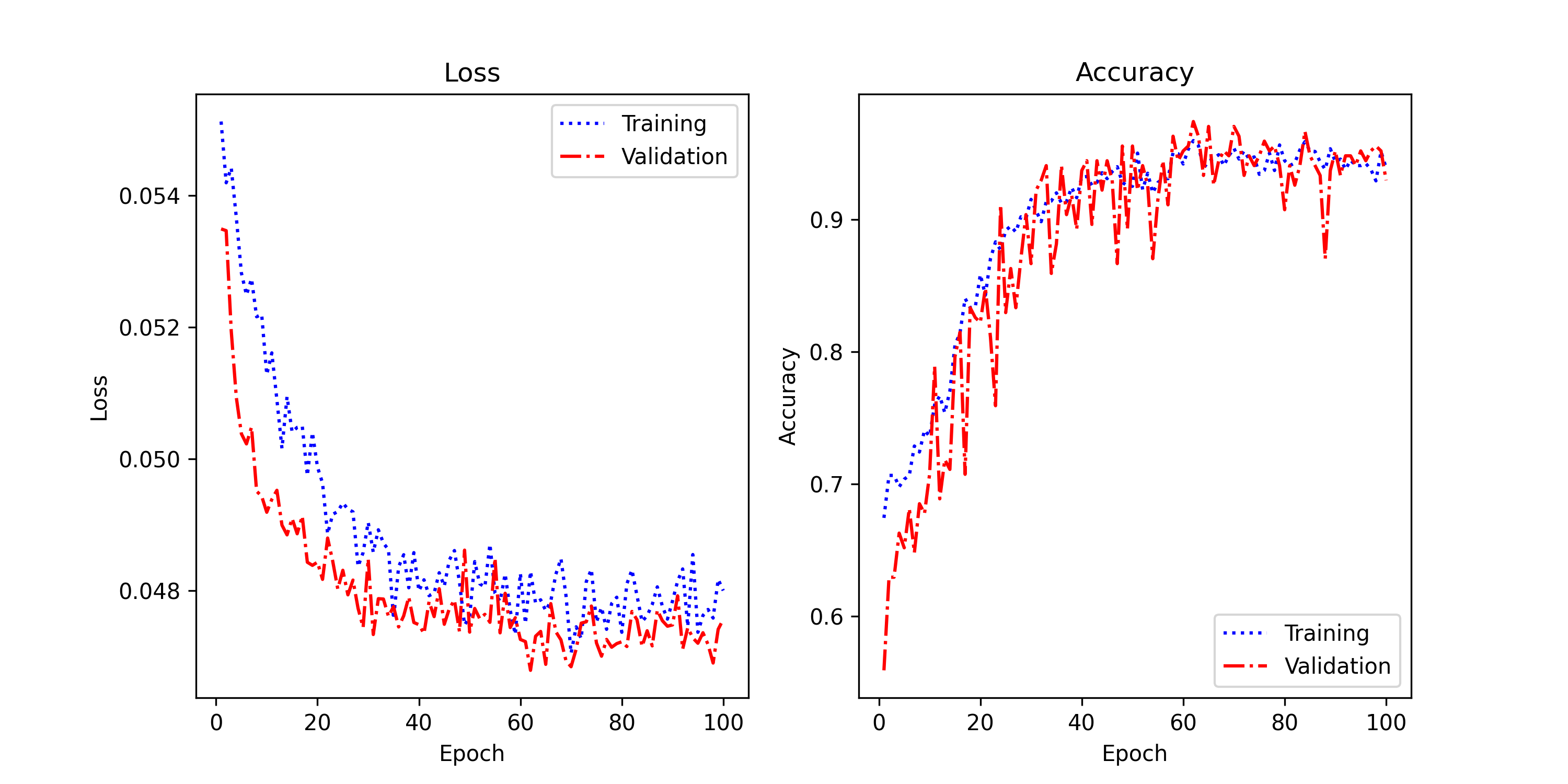
Loss & Accuracy Curves
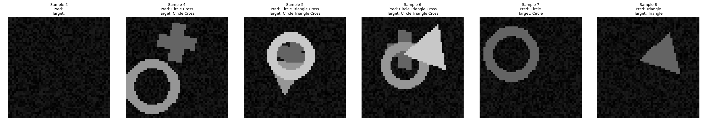
Tests on images show that the model recognizes shapes correctly. The main error cases correspond to overlapping shapes or partially visible shapes. Careful, shape-preserving augmentation may help, though aggressive transforms hurt performance on this dataset (see Section 3).
4.2 Object Detection
78.3% mAP means the model finds the right object in the right place about 4 times out of 5, within the strict parameter budget required for embedded deployment.
Detection achieves an mAP of 78.3%, showing good ability to locate and classify objects. However, fluctuations are visible on the validation set, suggesting potential instability and overfitting. Some bounding boxes are not perfectly aligned with the actual objects.
Loss & mAP Curves
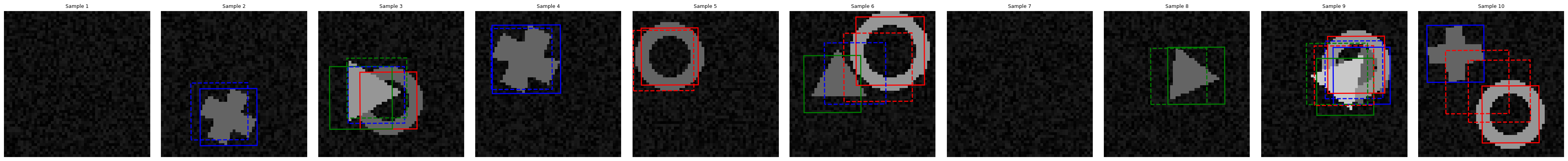
Detection Predictions
Results show some error cases: imperfect box alignment, shape classification errors, multiple detections of the same object. Improvements could come from revising the loss function or more aggressive data augmentation (random rotations).
4.3 Semantic Segmentation
86% IoU means the model correctly labels roughly 6 out of every 7 pixels, achieved with under 1 million parameters and fewer than 300 training images.
Semantic segmentation achieves a best validation IoU of 86.0% (epoch ~142), demonstrating the U-Net model's ability to accurately segment shapes at the pixel level. The final train IoU of 96.2% yields a train-val gap of ~10%, indicating moderate overfitting that stabilized after epoch 80. The architecture with skip-connections proves very effective for preserving contours.
Training ran for 150 epochs, with the model converging steadily from epoch 1 (IoU ~27%) to plateau around epoch 80–100 (IoU ~84–85%). Beyond epoch 100, improvements are marginal. The final validation loss of 0.00114 reflects stable and well-fitted training.
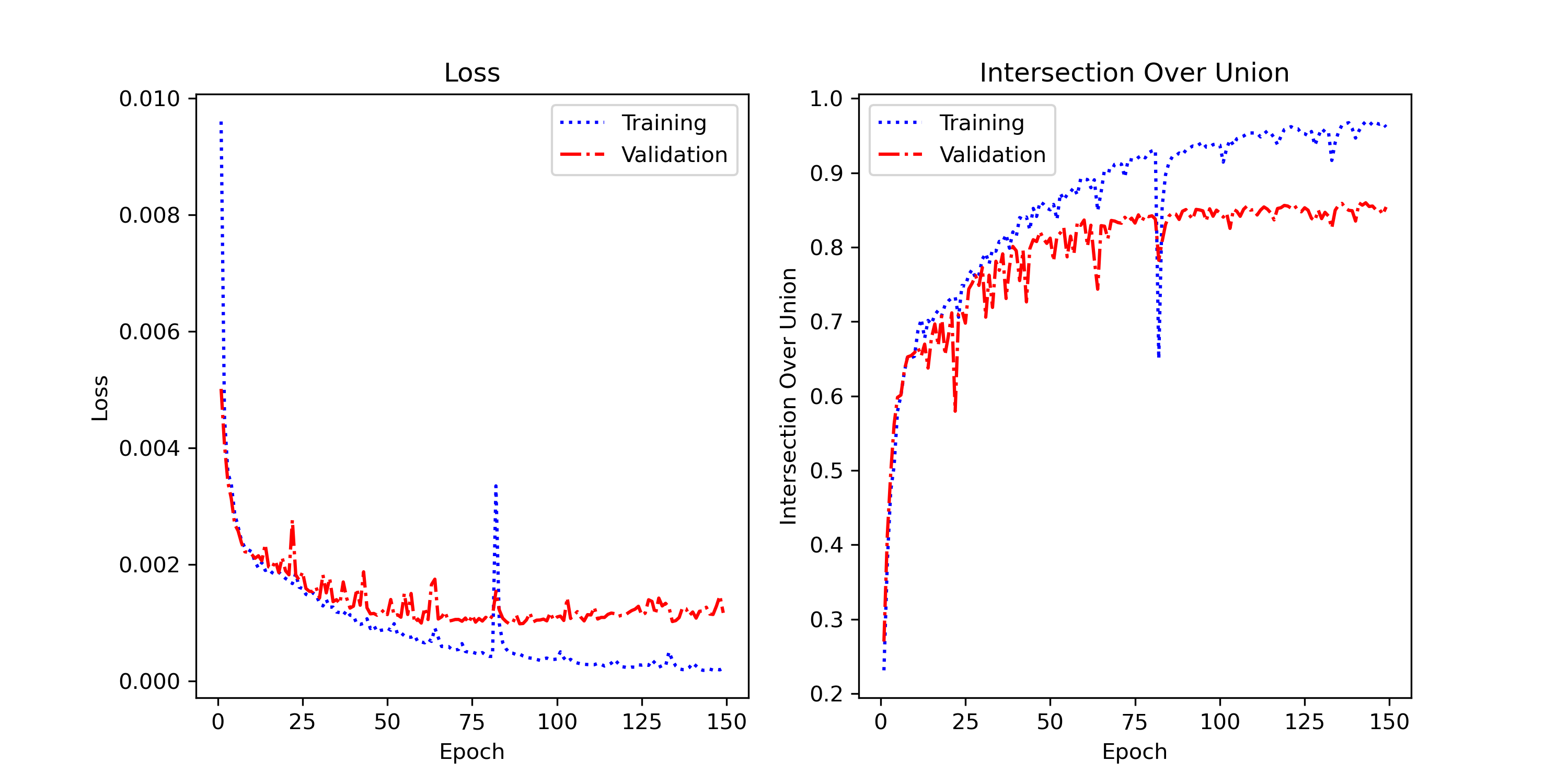
Loss & IoU Curves
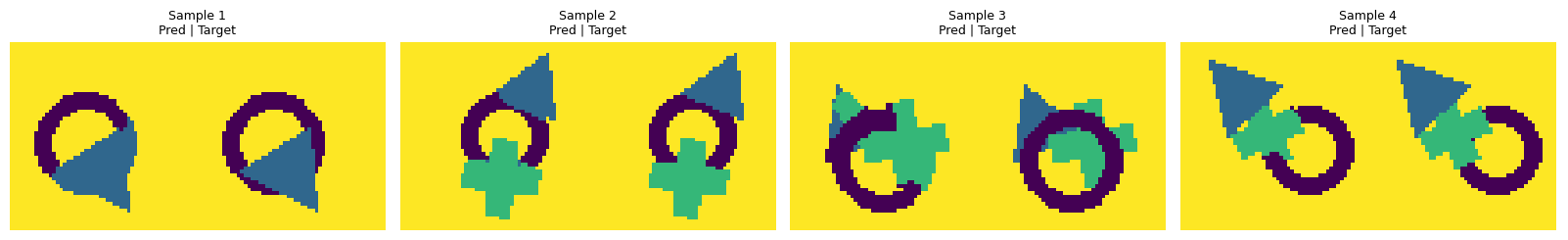
Tests on segmentation show that the model accurately delineates shape boundaries and generates precise pixel-level masks. The main error cases correspond to overlapping shapes where boundaries become ambiguous, and partially visible shapes at image edges. Performance can be improved through data augmentation (random rotations, zooms, and edge variations) to handle more diverse segmentation scenarios.
6. Conclusion & Future Perspectives
Project Summary
This project validated the feasibility of a proof of concept to automate scanner image processing through convolutional neural networks. The three developed architectures (classification, detection, segmentation) demonstrate that optimized models can achieve good performance even with strict resource constraints.
Key Successes
- Robust classification with 96.0% test accuracy on 100-sample test set
- Precise segmentation with 86.0% IoU using a compact U-Net with skip-connections
- All three models respect the parameter limits defined in the project constraints
- Acceptable inference time of ~14-18 ms for the full pipeline
- Modular and well-documented code that can be adapted for other image tasks
Key Learnings
- BatchNorm is essential for stability, especially in detection
- Skip-connections are crucial for preserving spatial information
- Adapting architecture to data is more important than using standard architectures unchanged
- Monitoring validation curves allows quick identification of overfitting problems
- Hyperparameter optimization must be iterative and based on curve observations
Future Improvements
- Test on Real Data: Validate on actual scanner images (domain transfer)
Resources & Links
View Complete Source Code on GitHubAssociated Documents
- Project Statement: Problematique_gro721_guide_etudiant_H25.pdf
- Source Code: Dataset, models, training scripts on GitHub